
前回の投稿で、pythonを使ってDICOMファイルを表示したり、MPRで表現しました。
今回は、skimageを使ってサーフェスレンダリングを実施します。マーチングキューブ法(marching cube)で骨の表面をmeshとして取り出し、OBJファイルで保存したいと思います。
前回の記事にて、DICOMファイルからNumpy arrayにする方法を書きました。コードだけ掲載しておきます。なお、当該DICOMデータは、rescale slopeが1でrescale interceptが0だったので、pixel valueを変換する必要はありませんでした。そのままpixel valueがCT値です。
import pydicom
import numpy as np
import matplotlib.pyplot as plt
import sys
import glob

# DICOM ファイルを読み込み
files = []
print('DICOMファイルの場所: {}'.format("C:\\Users\\patient_name/*"))
for fname in glob.glob("C:\\Users\\patient_name/*", recursive=False):
    files.append(pydicom.dcmread(fname))

# slicesというリストを作成。ファイルに、slicelocationという属性があれば追加していく。
slices = []
skipcount = 0
for f in files:
    if hasattr(f, 'SliceLocation'):
            if f.SeriesNumber==5: #5回CTを撮影し、5回目のデータのみを抽出
                slices.append(f)
    else:
        skipcount = skipcount + 1

print("該当ファイル数: {}".format(len(slices)))
print("スライス位置がないファイル: {}".format(skipcount))

# スライスの順番をそろえる
slices = sorted(slices, key=lambda s: s.SliceLocation) # .SliceLocationで場所情報を取得
# len(slices) = 270

# アスペクト比を計算する
ps = slices[0].PixelSpacing    # ps = [0.571, 0.571] 1ピクセルの [y, x] 長さ
ss = slices[0].SliceThickness  # ss = "3.0" スライスの厚み
ax_aspect = ps[0]/ps[1]        # yの長さ/xの長さ =  1
sag_aspect = ss/ps[0]          # スライスの厚み/y軸方向への1ピクセルの長さ = 3/0.571 = 5.25
cor_aspect = ss/ps[1]          # スライスの厚み/x軸方向への1ピクセルの長さ = 3/0.571 = 5.25

# 空の3Dのnumpy arrayを作成する
img_shape = list(slices[0].pixel_array.shape) # img_shape = [512, 512]
img_shape.insert(0,len(slices)) # img_shape = [270, 512, 512]
img3d = np.zeros(img_shape) # 空のarrayを作る np.zeros([270, 512, 512])

# 3Dのnumpy arrayを作る
for i, s in enumerate(slices):
    img2d = s.pixel_array    # img2d.shape = (512, 512)
    img3d[i,:, :] = img2d    # img3d.shape = (270, 512, 512)

# プロットする
middle0 = img_shape[0]//2  #3d array の(z軸)頭尾軸中央 270/2 = 135
middle1 = img_shape[1]//2  #3d array の(y軸)上下軸中央 512/2 = 256
middle2 = img_shape[2]//2  #3d array の(x軸)左右軸中央 512/2 = 256

a1 = plt.subplot(1, 3, 1)
plt.imshow(img3d[middle0,:, :])
a1.set_aspect(ax_aspect)  # ax_aspect = 1

a2 = plt.subplot(1, 3, 2)
plt.imshow(img3d[:, middle1, :])
a2.set_aspect(cor_aspect) # cor_aspect = 5.25

a3 = plt.subplot(1, 3, 3)
plt.imshow(img3d[:, :, middle2]) #
a3.set_aspect(sag_aspect) # sag_aspect = 5.25

plt.show()
現在、img3dという変数にnumpy arrayが入っています。
img3d.shape = (270, 512, 512)
このarrayの中には、CT値が入っています。
np.amin(img3d)-2048
np.amax(img3d)8908.0
CT値は、-2048 から 8908の数値を取っています。CT値は以下のような分布をしています。
| 骨 | 300 ~ 1000 |
| 軟部 | 30 ~ 50 |
| 脂肪 | -50 ~ -100 |
| 空気 | -1000 |
| 撮影範囲外 | -2048 |
体の中でCT値が大きいのは骨です。そのため、CT値が300以上のarrayを抽出していけば、骨の輪郭を取り出すことができます。
skimageというパッケージの中に、marching_cubesというメソッドがあります。これを使って、メッシュを取り出します。
使い方は、以下の通りです。
skimage.masure.marching_cubes(volume, level=None, spacing=(1.0, 1.0, 1.0), step_size=1, mask=None)
- volume: 3次元のNumpy arrayデータ。今回はimg3d。
- level: 領域内と領域外を分けるための数値を設定します。今回は、300以上を領域内とし、それ以下を領域外とするので299と設定します。
- spacing: ボクセルのサイズ。slices[0].SliceThickness=3.0、slices[0].PixelSpacing= [0.571, 0.571] の数値を入れます。
- step_size: デフォルトのまま1です。ステップを大きくすると、結果は速くなりますが、粗くなります。
- mask: 必須項目ではないので入れません。Bool型のvolumeと同じサイズのnumpy array。これにより、計算が早くなります。Trueのところだけ計算されるはず。
返り値は、4つあります。
verts, faces, normals, values = measure.marching_cubes()
verts(V, 3) 配列
V 個のユニークなメッシュ頂点の空間座標。
faces(F, 3) 配列
vertsから頂点インデックスを参照して三角形の面を定義します。
normals(V, 3) 配列
データから計算された各頂点の法線方向。
values(V, ) 配列
各頂点付近のローカル領域のデータの最大値。
以下がコードです。
import numpy as np
import matplotlib.pyplot as plt
from mpl_toolkits.mplot3d.art3d import Poly3DCollection
from skimage import measure

# マーチングキュープ法を実施
verts, faces, normals, values = measure.marching_cubes(img3d,
                                                     level=299,
                                                     spacing=(3,0.57, 0.57))

# Matplotlibを使って表示します。
fig = plt.figure(figsize=(10, 10))
ax = fig.add_subplot(111, projection='3d')

mesh = Poly3DCollection(verts[faces])
mesh.set_edgecolor('k')
ax.add_collection3d(mesh)

ax.set_xlabel("x-axis")
ax.set_ylabel("y-axis")
ax.set_zlabel("z-axis")

ax.set_xlim(0, 800)
ax.set_ylim(0, 800)
ax.set_zlim(0, 800)

plt.tight_layout()
plt.show()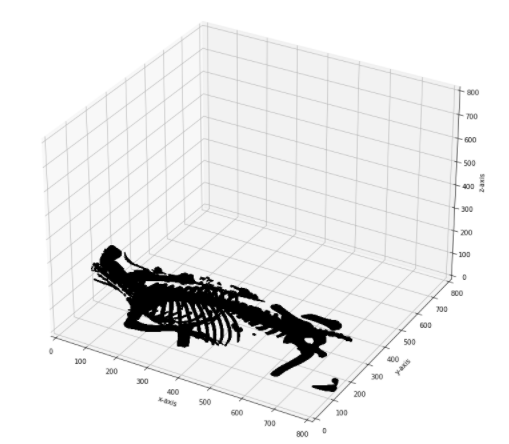
できました!ただ、matplotlibだとインタラクティブに回転しないのがネックですね。
実行に結構時間がかかるので、以下早くすることを目的としてmask配列を作ります。threshold配列はいらないといえばいらないですが、今後の勉強のために作ります。
DICOMのデータを格納したimg3dを編集します。
img3dのコピーを作り、CT値が300以上を2とし、300未満を0としたthreshold配列をつくります。また、maskを作ると計算が早くなるとのことなので、TrueとFalseだけのarrayを作成します。300以上をTrue、300未満をFalseにします。
import copy

# DICOMのデータが入ったimg3dをコピーし、名前をimg3d_thresholdとします。
img3d_threshold = copy.deepcopy(img3d)
# img3dと同じ形の0だけのnumpy arrayを作ります。dtype=boolとしてください。
img3d_boolean = np.zeros(img_shape, dtype=bool)

# CT値が300未満の場合
indice_under = img3d_threshold < 300
# img3d_thresholdに0を入れます。
img3d_threshold[indice_under] = 0
# img3d_booleanにfalseを入れます。
img3d_boolean[indice_under] = False

# CT値が300以上の場合
indice_over = img3d_threshold >= 300
# img3d_thresholdに2を入れます。
img3d_threshold[indice_over] = 2
# img3d_booleanにtrueを入れます。
img3d_boolean[indice_over] = True
import numpy as np
import matplotlib.pyplot as plt
from mpl_toolkits.mplot3d.art3d import Poly3DCollection
from skimage import measure
# マーチングキュープ法を実施
verts, faces, normals, values = measure.marching_cubes(img3d_threshold,
level=1,
spacing=(3,0.57, 0.57),
mask=img3d_boolean)
# グラフを作成
fig = plt.figure(figsize=(10, 10))
ax = fig.add_subplot(111, projection='3d')
mesh = Poly3DCollection(verts[faces])
mesh.set_edgecolor('k')
ax.add_collection3d(mesh)
ax.set_xlabel("x-axis")
ax.set_ylabel("y-axis")
ax.set_zlabel("z-axis")
ax.set_xlim(0, 800)
ax.set_ylim(0, 800)
ax.set_zlim(0, 800)
plt.tight_layout()
plt.show()少しばかり早くなったかな?
今度は、skimageで作ったメッシュを、OBJファイルに保存します。skimageにmeshを保存する機能がありません。
以下のコードでOBJファイルに保存できます。
faces = faces+1
thefile = open('DICOM_bone.obj', 'w')
for item in verts:
thefile.write("v {0} {1} {2}\n".format(item[0],item[1],item[2]))
for item in normals:
thefile.write("vn {0} {1} {2}\n".format(item[0],item[1],item[2]))
for item in faces:
thefile.write("f {0}//{0} {1}//{1} {2}//{2}\n".format(item[0],item[1],item[2]))
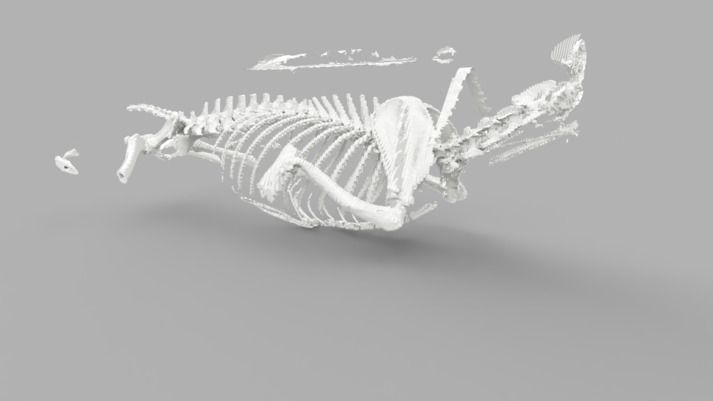
thefile.close()objファイルをFusion 360でレンダリングしました。

残すところは、ボリュームレンダリングです。これは、CT値のプロットを透過性を持たせて見せるという方法です。Jupyter notebookのせいかわかりませんが、plotlyでやろうとすると固まってしまいます。VTKを使ってやるのがよいようですが、学習には時間がかかりそうです。