基本的な統計・統計検定 in python

pythonでは多くの検定がscipyで実行することができます。多重検定に、statsmodels・scikit_posthocsを使用します。

まずはサンプルデータを作成

#groupAは平均５,分散５の正規分布　サンプル数3000
#groupBは平均３,分散３の正規分布　サンプル数3000
import numpy as np
group_a = np.random.normal(loc = 5, scale = 5, size = 3000)
group_b = np.random.normal(loc = 3, scale = 3 ,size = 3000)
#pandas dataframeにする
import pandas as pd
df = pd.DataFrame([group_a,group_b]).T
df.columns = ["groupA","groupB"]
df.head()

　　 groupA groupB
0　4.352208　2.398484
1　0.544291　-0.282820
2　7.192572　5.239167
3　5.584534　-0.485194
4　5.316293　-1.733356

ヒストグラムで分布を見てみる

import seaborn as sns
sns.set_palette("Pastel2")
sns.histplot(df)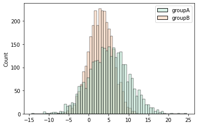

１. 連続値　母平均の推定

グループAの母平均の推定をしてみる。scipy statsのt.intervalを使う。

from scipy import stats
# stats.t.interval(信頼水準,
#                 自由度（= サンプルサイズ-1),
#                 標本平均,
#                 標準誤差)
stats.t.interval(alpha=0.95,
                 df = len(df["groupA"])-1,
                 loc = df["groupA"].mean(),
                 scale = stats.sem(df["groupA"]))

(4.669752163024685, 5.0280537828945855)

グループAの母平均は、4.67 – 5.02の間に95%の確率で存在すると推定できた。

なお標準誤差の求め方は、以下のどれでもよい。

from scipy import stats
from numpy as np
print(stats.sem(df["groupA"]))
print(np.sqrt(df["groupA"].var()/len(df["groupA"])))
print(df["groupA"].std()/np.sqrt(len(df["groupA"])))

0.09136826414810341
0.09136826414810341
0.09136826414810341

ブートストラップ法による母平均の推定もできる。ブートストラップとは、サンプル内からサンプリングを繰り返し多数の群を作成し、その多数の群の統計値の分布を計算する方法。

from scipy import stats
# Compute a two-sided bootstrap 
# confidence interval of a statistic.
stats.bootstrap([df["groupA"]],
                statistic= np.mean,
                confidence_level = 0.95)

BootstrapResult(confidence_interval=ConfidenceInterval(low=4.670533950615315, high=5.0267556892931635), standard_error=0.09072654647457754)

母平均の値は4.67 – 5.03（信頼区間95％）となり、さきほどのｔ分布を使用した結果とほぼ同じ。

検定の前提条件をチェック

２群の差の検定をする際に、どの検定方法がよいのか検討する。その際に、以下２点が選択する際の基準になる。
①それぞれの群が正規分布しているのか
　　shapiro wilk test
②２群は等しい分散なのか　　
　　F-test (pythonに実装なし)
　　bartlett（正規分布の仮定あり）
　　levene （仮定なし）

ただ、ものの本によるとこれらの検定を重ねて、最終的に２群の差の検定をすることは過誤を起こしやすくなっていて、いきなり仮定のない検定をしたほうがいいと言われ始めているようだ。（例：studentTよりwelchTtest)

正規分布のテスト　Shapiro-Wilk test

The Shapiro-Wilk test tests the null hypothesis that the data was drawn from a normal distribution.

from scipy import stats
print(stats.shapiro(df["groupA"]))
print(stats.shapiro(df["groupB"]))

ShapiroResult(statistic=0.9995990991592407, pvalue=0.8339430689811707) ShapiroResult(statistic=0.9991313815116882, pvalue=0.15253688395023346)

null hypoは正規分布から取ってきたものであることなので、それぞれ棄却失敗したのでgroupAとgroupBは正規分布ということがわかる。

２群は等しい分散なのか

scipyのページによると、bartletテストよりleveneテストの方がいい場合（正規分布でない場合）があるそうなので、leveneテストだけを使うようにする。

Bartlett’s test tests the null hypothesis that all input samples are from populations with equal variances. For samples from significantly non-normal populations, Levene’s test levene is more robust.

The Levene test tests the null hypothesis that all input samples are from populations with equal variances. Levene’s test is an alternative to Bartlett’s test bartlet in the case where there are significant deviations from normality.

from scipy import stats
stats.levene(df["groupA"],df["groupB"],center='mean')

LeveneResult(statistic=631.0326630284198, pvalue=1.719031499878635e-132)

null hypoは２群が等分散なので、棄却したのでgroupAとgroupBは等分散ではない。（groupAは分散5、groupBは分散3で作ったデータなので正しい）

これまでの検定の結果からは、グループAとBは正規分布で、グループAとBは分散が等しくないことから、グループAとグループBの平均の差の検定にはWelch’s t-testを用いるのが適当となります。

2群の平均値の差の検定(正規分布を仮定)

対応のない場合 等分散      student T test

今回のgroupAとgroupBは等分散ではなかったので、このテストを用いるのは正しくないが、正しかった場合は以下のコードとなる。

from scipy import stats
stats.ttest_ind(df["groupA"], df["groupB"], equal_var=True)

Ttest_indResult(statistic=16.634821499213523, pvalue=8.82318870294875e-61)

2群の間に平均の差がないという仮説を棄却失敗　→　2群に平均の差がある

対応のない場合 等分散の仮定なし　welch t test

from scipy import stats
stats.ttest_ind(df["groupA"], df["groupB"], equal_var=False)

Ttest_indResult(statistic=16.63482149921352, pvalue=1.762129440616374e-60)

2群の間に平均の差がないという仮説を棄却失敗　→　2群に平均の差がある

2群の代表値の差の検定(正規分布を仮定しない)

対応のない場合　Mann-Whitney U rank test

The Mann-Whitney U test is a nonparametric test of the null hypothesis that the distribution underlying sample x is the same as the distribution underlying sample y.

from scipy import stats
stats.mannwhitneyu(df["groupA"],df["groupB"])

MannwhitneyuResult(statistic=5700020.0, pvalue=1.4799651035379324e-71)

分布がグループAとグループBで違うので、２群には差がある。

対応のない場合 Wilcoxon rank-sum test

The Wilcoxon rank-sum test tests the null hypothesis that two sets of measurements are drawn from the same distribution. The alternative hypothesis is that values in one sample are more likely to be larger than the values in the other sample.

This test should be used to compare two samples from continuous distributions. It does not handle ties between measurements in x and y. For tie-handling and an optional continuity correction see scipy.stats.mannwhitneyu.

from scipy import stats
stats.ranksums(df["groupA"],df["groupB"])

RanksumsResult(statistic=17.887351411881344, pvalue=1.4797672048790702e-71)

２群が同じ分布からサンプルされた確率がp値なので、棄却。

3群の平均値の比較

・３群のそれぞれが正規分布かつ等分散であれば
　　ANOVA（差の検定）→　
　　Tukey’S HSD test（多重検定）

３群のデータのサンプルを作成する

import numpy as np
import pandas as pd
g_a = np.random.normal(loc=5, scale=5.0, size=3000)
g_b = np.random.normal(loc=4.5, scale=4 ,size = 3000)
g_c = np.random.normal(loc=4.5, scale=5, size = 3000)
df = pd.DataFrame([g_a, g_b, g_c]).T
df.columns = ["groupA","groupB","groupC"]

ANOVAをするにあたっては、正規分布のチェックと３群の等分散のチェックをする。

正規性のチェック

for column in df:
    print( f" {column} is tested by shapiro", stats.shapiro(df[column]))

groupA is tested by shapiro ShapiroResult(statistic=0.9995654225349426, pvalue=0.7768710255622864)
groupB is tested by shapiro ShapiroResult(statistic=0.9990720748901367, pvalue=0.11586038023233414)
groupC is tested by shapiro ShapiroResult(statistic=0.9995706081390381, pvalue=0.7859545350074768)

すべて正規分布がわかった。

３群の等分散のチェック

from scipy import stats
stats.levene(df["groupA"],df["groupB"],df["groupC"])

LeveneResult(statistic=77.8389348495974, pvalue=3.0487292789522742e-34)

等分散でないことが分かった。

３群は正規分布だったが、等分散ではなかったことからANOVAは不適だが、実行してみる。

ANOVA（正規分布かつ等分散のとき）

The one-way ANOVA tests the null hypothesis that two or more groups have the same population mean. The test is applied to samples from two or more groups, possibly with differing sizes.

from scipy import stats
stats.f_oneway(df["groupA"],df["groupB"],df["groupC"])

F_onewayResult(statistic=16.83482783350308, pvalue=5.039340392005426e-08)

３群の平均値は異なるという結果がでた。それでは、どの群とどの群に差があったのか調べたいと思う。

Tukey’S HSD test（多重検定）

statsmodelを使用する

import statsmodels.api as sm
endog = df.values
endog  = np.ravel(endog)
groups = np.tile(["groupA","groupB","groupC"],len(df))   
print(sm.stats.multicomp.pairwise_tukeyhsd(endog,groups,alpha=.05))

Multiple Comparison of Means - Tukey HSD, FWER=0.05 
 group1 group2 meandiff p-adj   lower   upper  reject
 groupA groupB  -0.5446  0.001 -0.8295 -0.2597   True
 groupA groupC  -0.6604  0.001 -0.9453 -0.3755   True
 groupB groupC  -0.1158 0.5985 -0.4007  0.1691  False

・３群のそれぞれが正規分布かつ等分散という仮定をしない場合
　　Kruskal-Wallis test（差の検定） →
　　Dunn’s test（多重検定）

Kruskal-Wallis test

The Kruskal-Wallis H-test tests the null hypothesis that the population median of all of the groups are equal.

from scipy import stats
stats.kruskal(df["groupA"],df["groupB"],df["groupC"])

KruskalResult(statistic=34.16578118470352, pvalue=3.810613316339335e-08)

中央値が同じという仮定を棄却された。（＝中央値に差がある）

Dunn’s test

scikit-posthocsというパッケージを使用します。

Post hoc pairwise test for multiple comparisons of mean rank sums (Dunn’s test). May be used after Kruskal-Wallis one-way analysis of variance by ranks to do pairwise comparisons

!pip install -q scikit_posthocs

読み込ませる形に整えるためにmeltを使用します。

df_melted = df.melt()
df_melted

　　variable 　value
0 　groupA 　-2.324726
1 　groupA 　7.607998
2 　groupA 　11.247948
3 　groupA 　6.143492
4 　groupA 　6.638160

Dunn’s testを実行します。

import scikit_posthocs
df_melted = df.melt()
scikit_posthocs.posthoc_dunn(df_melted,val_col="value",group_col="variable")

　　　　　　　groupA 　　groupB 　　　groupC
groupA 　1.000000e+00 　0.000003 　7.118960e-08
groupB 　3.219688e-06 　1.000000 　4.642545e-01
groupC 　7.118960e-08 　0.464255 　1.000000e+00

groupBとgroupCが同じだとされました。以下、サンプルを作成したときのコードです。たしかにBとCは似ています。

g_a = np.random.normal(loc=5, scale=5.0, size=3000)
g_b = np.random.normal(loc=4.5, scale=4 ,size = 3000)
g_c = np.random.normal(loc=4.5, scale=5, size = 3000)

2.確率

まずはデータを作成

from scipy.stats import binom
# binom.rvs(出てくる数字の最大値,
#           ０　～　出てくる数字の最大値　のどこが最頻になるか,
#           取り出すサンプルの量)
groupA = binom.rvs(1, 0.5, size=1000)
groupB = binom.rvs(1, 0.3, size=1000)
import pandas as pd
df = pd.DataFrame([groupA,groupB]).T
df.columns = ["groupA","groupB"]
print(df["groupA"].sum()/len(df)) #0.478
print(df["groupB"].sum()/len(df)) #0.304

母比率の推定

方法１ statsmodelsを使用

from statsmodels.stats.proportion import proportion_confint
proportion_confint(count=df["groupA"].sum(), nobs=len(df))

(0.44704026099747746, 0.5089597390025226)

方法２　scipyを使用

from scipy.stats import binomtest
res = binomtest(500, 1000).proportion_ci()
print(res)
print(res.high)
print(res.low)

ConfidenceInterval(low=0.46854917297179194, high=0.531450827028208)
0.531450827028208
0.46854917297179194

from scipy.stats import binom
low,high = binom.interval(alpha=0.95, n=len(df), p=df["groupA"].sum()/len(df), loc=0)
print(f"low:{low/len(df)}, high:{high/len(df)}") 

low:0.447, high:0.509

2群の比率の検定　カイ二乗検定

from scipy import stats
import pandas as pd
temp = pd.DataFrame({
    "a":[20 , 100 - 20],
    "b":[40 , 100 - 40]
})
stats.chi2_contingency(temp).pvalue

0.0033704314473977145

（以下　カイ二乗検定について古い記述）

2 x 2 Contingency Tableを作るためには、一回メルトが必要

df_melted = df.melt()
contingency = pd.crosstab(df_melted["value"], df_melted["variable"])
contingency 

variable  groupA  groupB
value        
 0     　 　522      696
 1      　　478      304

Chi-square test of independence of variables in a contingency table.

This function computes the chi-square statistic and p-value for the hypothesis test of independence of the observed frequencies in the contingency table observed.  This is a test for the independence of different categories of a population. The test is only meaningful when the dimension of observed is two or more.

from scipy import stats
print(stats.chi2_contingency(contingency , correction=False))

(63.57325538911216, 1.5451273468690328e-15, 1, array([[609., 609.], [391., 391.]]))

(chi2float, pfloat, dofint, expectedndarray)

chi2float:The test statistic.
pfloat: The p-value of the test
dofint: Degrees of freedom
expectedndarray, same shape as observed: The expected frequencies, based on the marginal sums of the table.

p値は0.05以下なので、２群は独立だという結果になった。

3群の比率の検定　カイ二乗検定　→　post hoc test

from scipy.stats import binom
groupA = binom.rvs(1, 0.33, size=1000)
groupB = binom.rvs(1,0.3,size=1000)
groupC = binom.rvs(1,0.25,size=1000)
import pandas as pd
df = pd.DataFrame([groupA,groupB,groupC]).T
df.columns = ["groupA","groupB","groupC"]
df["groupA"].sum()/len(df)
df["groupB"].sum()/len(df)
df["groupC"].sum()/len(df)
df_melted = df.melt()
contingency = pd.crosstab(df_melted["value"], df_melted["variable"])
contingency
from scipy import stats
print(stats.chi2_contingency(contingency , correction=False))
# (chi2float, pfloat, dofint, expectedndarray)

(22.008260368157977, 1.663286194795178e-05, 2, array([[699.66666667, 699.66666667, 699.66666667], [300.33333333, 300.33333333, 300.33333333]]))

p値が0.5以下なので、3群の比率は同じではないという結果です。

Post hoc test

statsmodelsの中にあるmultipletestsを使用してp値を修正する関数を定義。

def posthoc_test_after_chisq(crosstable): 
     
  from itertools import combinations
  all_combinations = list(combinations(df.columns, 2))
  raw_pvalues = []
    
  from scipy.stats import chi2_contingency
  for comb in all_combinations:
    _, p, _, _ = chi2_contingency(crosstable.filter(comb), correction=True)
    raw_pvalues.append(p)
    
    from statsmodels.stats.multitest import multipletests
    rejectndarray, pvals_correctedndarray, _ , _ = multipletests(raw_pvalues, method='bonferroni')  
    # rejectndarray, bool:    true for hypothesis that can be rejected for given alpha
    # pvals_correctedndarray: p-values corrected for multiple tests
    # alphacSidakfloat:       corrected alpha for Sidak method
    # alphacBonffloat:        corrected alpha for Bonferroni method
    # method can be: bonferroni, sidak, holm-sidak, holm, simes-hochberg, hommel, fdr_bh, fdr_by, fdr_tsbh, fdr_tsbky
    
    for raw_p_val, corr_p_val, reject, comb in zip(raw_pvalues, pvals_correctedndarray, rejectndarray, all_combinations):
      print(f"{comb}: raw_p_value: {raw_p_val:.3f}; corrected: {corr_p_val:.3f} null-hypo-reject: {reject}")

posthoc_test_after_chisq(contingency)

(‘groupA’, ‘groupB’): raw_p_value: 0.739; corrected: 1.000 null-hypo-reject: False
(‘groupA’, ‘groupC’): raw_p_value: 0.000; corrected: 0.000 null-hypo-reject: True
(‘groupB’, ‘groupC’): raw_p_value: 0.000; corrected: 0.000 null-hypo-reject: True

groupAとC、groupBとCが異なる、groupAとBは同じという結果でした。

groupA = binom.rvs(1, 0.33, size=1000)
groupB = binom.rvs(1,0.3,size=1000)
groupC = binom.rvs(1,0.25,size=1000)

3.比率調査のための必要サンプル数

予測される有病率 = 0.05
希望する絶対精度 = 0.05
print( round((1.96**2)*予測される有病率*(1-希望する絶対精度)/(希望する絶対精度**2)))

73