機械学習でワインの評価を予想
人によるワインの評価を、ワインの化学的分析の結果をもとに機械学習AIを使って予測したいと思います。医療・獣医療においても、病気の診断などで応用できると思います(データセットの入手が限られています)。
今回はRを使って、regression、decision tree、random forest、neural network、gradient boost machineを使ってワインの評価を予測します。10回ブートストラップを実施し、Mean Squared Errorを評価基準として一番いいモデルを選びます。その後、化学的性質のどういった因子が評価に重要かを調べます。
ワインのデータセットはUCI Machine learning repositoryから入手します。
https://archive.ics.uci.edu/ml/datasets/Wine+Quality
UCI機械学習リポジトリ:1987年にカリフォルニア大学アーバイン校のDavid Ahaと大学院生の仲間によってftpアーカイブとして作成されました。
ワインデータセット
ポルトガル北部の赤と白のヴィニホ・ベルデワインのサンプルに関連する2つのデータセットが含まれている。目的は、物理化学的試験に基づいてワインの品質をモデル化することである。
説明変数(物理化学的試験)
1 – 固定酸度
2 – 揮発性の酸度
3 – クエン酸
4 – 残糖
5 – 塩化物
6 – 遊離二酸化硫黄
7 – 全二酸化硫黄
8 – 密度
9 – pH
10 – 硫酸塩
11 – アルコール
目的変数(感覚データ)
12 – 品質(0から10の間のスコア)
白ワインのデータを使います。まずは下準備。
library(tidyverse) # グラフやデータ操作系
library(rpart) # decision tree
library(caret) # random forest, Neaural Network, Gradient Boost machine
library(gbm) # gradient boost machine
library(broom) # regressionでcoefの結果をdataframeにする
library(patchwork) # ggplot同士を結合する
library(GGally) # 相関グラフ化

library(doParallel) # CPUコアを全部使って高速化
cl <- makePSOCKcluster(4)
registerDoParallel(cl)

df_r <- read.delim("winequality-white.csv",sep=";")
MSEを計算するfunctionを作成します。
mse = function(true, predict){
  mean( (true-predict)^2  )
}
cross validationの結果を保存するための6列の空のデータフレームを作ります。
n <- 6
msedf <- data.frame(matrix(rep(NA, n), nrow=1))[numeric(0), ]
colnames(msedf) <- c("Regression",
                     "Scaled_regression",
                     "Tree",
                     "Random_forest",
                     "Neural_network",
                    "Gradient_boost_machine")
10回bootstrapを実施します。train test splitの比率は8:2です。
id <- seq(1,nrow(df_r), by = 1) # 1からデータサイズまでの数列
test_n <- floor(nrow(df_r)*0.2) # テストサイズを計算

for(i in 1:10){
# train test split
set.seed(i)
test_id <- sample(id, replace=F, size = test_n)
traindf <- df_r[-test_id,]
testdf <- df_r[test_id,]

# regression
reg <- lm(quality~.,
          data = traindf)

# standardized partial regression(標準化偏回帰)
traindf_scale <- as_tibble(scale(traindf))
traindf_scale <- traindf_scale %>% select(-quality)
traindf_scale$quality <- traindf$quality
reg_scale <- lm(quality~.,
                data = traindf_scale)
# decision tree
tree <- rpart(quality~.,
              data =traindf)
# 以下caret package。
# パラメータ設定(cross validation、進捗書き出し)しておく。
trainctrl <- trainControl(method = "cv", verboseIter = TRUE)

# random forest
forest <- train(quality~.,
                data =traindf,
                method="rf",
                preProcess = c("center", "scale"),
                importance = TRUE,
                trControl = trainctrl)
# neural network
NN <- train(quality~.,
            data =traindf,
            method="nnet",
            preProcess = c("center", "scale"),
            importance = TRUE,
            linout = TRUE,
            trControl = trainctrl)
# gradient boost machine
gbm <- train(quality~.,
             data =traindf,
             method="gbm",
             preProcess = c("center", "scale"),
             trControl = trainctrl)
# 結果の保存
msedf[i,1]  <- mse(testdf$quality, predict(reg, newdata=testdf))
msedf[i,2]  <- mse(testdf$quality, predict(reg_scale, newdata=as_tibble(scale(testdf))))
msedf[i,3]  <- mse(testdf$quality, predict(tree, newdata = testdf))
msedf[i,4]  <- mse(testdf$quality, predict(forest, newdata = testdf))
msedf[i,5]  <- mse(testdf$quality, predict(NN, newdata = testdf))
msedf[i,6]  <- mse(testdf$quality, predict(gbm, newdata = testdf))
}
# 10回のMSE平均を計算
result <- tibble(Mean_MSE = colMeans(msedf),
                 Method = colnames(msedf))
# 小数点を丸める
result$Mean_MSE <- round(result$Mean_MSE, digits = 2)
# グラフ化
ggplot(result) +
  geom_bar(stat = "identity", aes(x = Method, y=Mean_MSE,fill=Method)) +
  geom_text(aes(x = Method, y=Mean_MSE,label = Mean_MSE), vjust=1.6, color="black", size=5) +
  scale_fill_brewer(palette = "Set3") +
  coord_flip()+
  theme_minimal()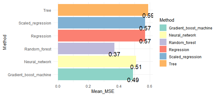
Random Forestが1番いいモデルだということが分かりました。実際のスコアと予想スコアの差の2乗の平均が0.37なので、正答率は高いです。改めてRandom forest、1つのtrainデータセットを学習させ、確率からクラスを予想してAccuracyを計測してみます。
id <- seq(1,nrow(df_r), by = 1)
test_n <- floor(nrow(df_r)*0.2)
set.seed(123)
test_id <- sample(id, replace=F,size = test_n)

traindf <- df_r[-test_id,]
testdf <- df_r[test_id,]

forest <- train(quality~.,
                data =traindf,
                method="rf",
                preProcess = c("center", "scale"),
                importance = TRUE,
                trControl = trainctrl)

pred_forest <- predict(forest,
                       newdata = testdf)
pred_forest <- round(pred_forest, 0)
confmatrix <- as_tibble(table(true=testdf$quality, pred = pred_forest))
sum(confmatrix$n[confmatrix$true==confmatrix$pred])/
sum(confmatrix$n)
Accuracy: 0.67でした。random forestを使えば、7割近くの精度で正解を予想できることができることがわかりました!
ランダムに推測すると、10クラスを推測するのでAccuracy:0.1なので成績はまずまずというところです。
おまけで、変数の重要性を見てみます。
plot(varImp(forest))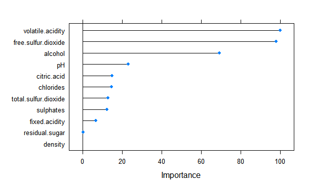
volatile.acidity(揮発性の酸度)、free.sulfur.dioxide(遊離二酸化硫黄)、alcohol(アルコール)が重要だとわかりました。重要性だけだと、評価に対してマイナスなのかプラスなのか、わからないのでregressionも実施したいと思います。変数のスケールが違うので、scaleした場合としない場合の両方を実施してみました。
reg <- lm(quality~.,
          data = traindf)

traindf_scale <- as_tibble(scale(traindf))
traindf_scale <- traindf_scale %>% select(-quality)
traindf_scale$quality <- df_r$quality
reg_scale <- lm(quality~.,
                data = traindf_scale)

co_logi <- tidy(reg, conf.int = FALSE)
co_logi <- co_logi %>% filter(term != "(Intercept)")
co_logi_scale <- tidy(reg_scale, conf.int = FALSE)
co_logi_scale <- co_logi_scale %>% filter(term != "(Intercept)")

g1 <- ggplot(co_logi, aes(x=term, y=estimate,fill=estimate) )+
  geom_bar(stat="identity")+
  coord_flip()+ggtitle("regression coefficient")+
  scale_fill_gradient(low="blue",high="pink")+
  theme_minimal()
g2 <- ggplot(co_logi_scale, aes(x=term, y=estimate,fill=estimate) )+
  geom_bar(stat="identity")+
  coord_flip()+ggtitle(" standardized regression coefficient")+
  scale_fill_gradient(low="blue",high="pink")+
  theme_minimal()
g1/g2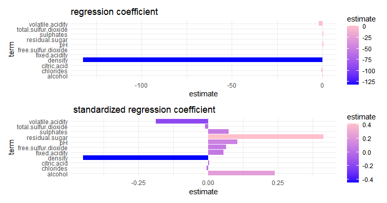
volatile.acidity(揮発性の酸度)はマイナスファクターだとわかりました。これを減らすのが重要ということでしょう。free.sulfur.dioxide(遊離二酸化硫黄)、alcohol(アルコール)はプラスファクターです。これらを増やすことが重要のようです。
ちなみに、regressionによるimportanceも見てみます。coefientの大きさとは関係ない事がわかります。
impreg <- varImp(reg)
g3 <- ggplot(data= impreg, aes(x=rownames(impreg),y=Overall)) +
  geom_bar(position="dodge",stat="identity",width = 0, color = "black") +
  coord_flip() + geom_point(color='skyblue') + xlab(" Importance Score")+
  ggtitle("Variable Importance") +
  theme(plot.title = element_text(hjust = 0.5)) +
  theme(panel.background = element_rect(fill = 'white', colour = 'black'))+
  ggtitle("regression")

impreg_scale  <- varImp(reg_scale)
g4 <- ggplot(data= impreg_scale, aes(x=rownames(impreg_scale),y=Overall)) +
  geom_bar(position="dodge",stat="identity",width = 0, color = "black") +
  coord_flip() + geom_point(color='skyblue') + xlab(" Importance Score")+
  ggtitle("Variable Importance") +
  theme(plot.title = element_text(hjust = 0.5)) +
  theme(panel.background = element_rect(fill = 'white', colour = 'black'))+
  ggtitle("standardized partial regression")

g3+g4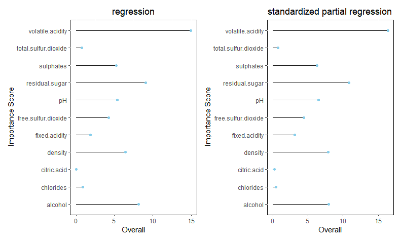
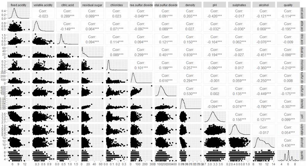
最後は、相関係数を見て全体をみて終わります。
library(GGally)
ggpairs(df_r)