LDAでカテゴリー予想 in R

on 2月 5, 2021

LDAは、教師あり学習の１つです。カテゴリ予想に使えます。logistic regressionとLDAの使い分けはlogistic regressionは通常２カテゴリの予想に使われるのに対して、LDAは３カテゴリー以上の予想に使われます。

教師あり学習 -logistic regressionでカテゴリ予想-

LDAの使い方を見てみます。使うデータは、デフォルトのirisデータです。必要なパッケージは、MASSです。

実践

library(MASS)
myiris <- iris
colnames(myiris)

[1] “Sepal.Length”
[2] “Sepal.Width”
[3] “Petal.Length”
[4] “Petal.Width”
[5] “Species”

irisにはカテゴリが３つあります。

table(myiris$Species)

setosa versicolor  virginica 
    50         50         50

さっそく、LDAを適用させます。

lda(式, data = データ）

lda <- lda(Species~.,
           data = myiris)

モデルが作れたので、モデルを使って予想したいと思います。

predict(モデル,　newdata = 予測したいデータ）

pred <- predict(lda,
                newdata = myiris)

predには何が入っているでしょうか。

pred$posterior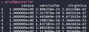

それぞれのクラスに分類される確率が入っていました。

pred$class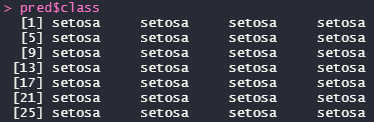

予想されるカテゴリーが入っていました。

pred$x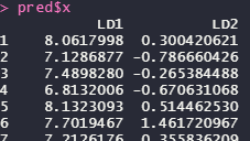

LDAの計算でつかわれる判別係数です。PCAみたいですね。

グラフを書いてみます。

library(tidyverse)

tibble(LD1 = pred$x[,1],
       LD2 = pred$x[,2],
       class = pred$class)%>% 
  ggplot()+
  geom_point(aes(x=LD1,y=LD2,color=class))+
  geom_density2d(aes(x=LD1,y=LD2),color="grey")+
  theme_minimal()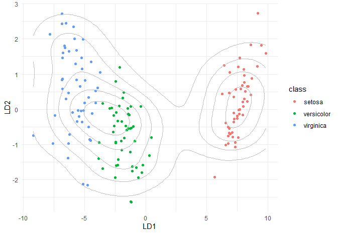

綺麗に分けられていますね。

accuracyを見てみます。


table(true=myiris$Species,
      prediction = pred$class)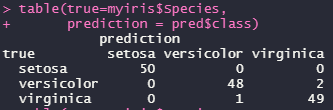

Accuracy = (50+48+49)/(50+48+1+2+49) = 0.98

なかなかいい成績ですね！

Categories:

実践

category