基礎的な統計 in R

たまに必要となる基礎的な統計についてメモ

１．母平均の推定

t.test(c(10,20,10,5,10))

One Sample t-test
data: c(10, 20, 10, 5, 10)
t = 4.4907, df = 4, p-value = 0.0109
alternative hypothesis: true mean is not equal to 0
95 percent confidence interval:
4.199126 17.800874
sample estimates:
mean of x
11

２．母比率の推定

binom.test(10,100) # 100個のうち10個

Exact binomial test
data: 10 and 100
number of successes = 10, number of trials = 100, p-value <
2.2e-16
alternative hypothesis: true probability of success is not equal to 0.5
95 percent confidence interval:
0.04900469 0.17622260
sample estimates:
probability of success
0.1

３．平均の差の検定

３－１－１
２群差検定　正規分布 かつ等分散　Students T-test

library(tidyverse)
value <- c(5,6,4,6,8,2,3,1,7,9)
group <- c("a","a","a","a","a","b","b","b","b","b")
df <- tibble(value,group)
t.test(value~group,data=df,var.equal=TRUE)

Two Sample t-test
data: value by group
t = 0.83666, df = 8, p-value = 0.4271
alternative hypothesis: true difference in means is not equal to 0
95 percent confidence interval:
-2.458683 5.258683
sample estimates:
mean in group a mean in group b
5.8 4.4

解釈：p-valueが0.05以下なら平均に差がある

２群差検定　正規分布 かつ非等分散　Welchのt検定

# Students T-test 
library(tidyverse)
value <- c(5,6,4,6,8,2,3,1,7,9)
group <- c("a","a","a","a","a","b","b","b","b","b")
df <- tibble(value,group)
t.test(value~group,data=df)

Welch Two Sample t-test
data: value by group
t = 0.83666, df = 5.4414, p-value = 0.438
alternative hypothesis: true difference in means is not equal to 0
95 percent confidence interval:
-2.798542 5.598542
sample estimates:
mean in group a mean in group b
5.8 4.4

解釈：p-valueが0.05以下なら平均に差がある

３－１－２
２群差検定（非正規分布）Wilcoxon rank-sum test

value <- c(5,6,4,6,8,2,3,1,7,9)
group <- c("a","a","a","a","a","b","b","b","b","b")
df <- tibble(value,group)
wilcox.test(value~group,data=df)

Wilcoxon rank sum test with continuity correction
data: value by group
W = 16, p-value = 0.5296
alternative hypothesis: true location shift is not equal to 0

解釈：p-valueが0.05以下なら平均に差がある

３－２－１
３群以上（正規分布） かつ（等分散）ANOVA

value <- c(5,6,4,6,8,2,3,1,7)
group <- c("a","a","a","b","b","b","c","c","c")
df <- tibble(value,group)
summary(aov(value~group,data=df))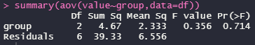

解釈：Prが0.05以下なら平均に差がある

ANOVAの後、どの群に差があったのかを調べる
Tukey’S HSD test　or　Pairwise t-test

Tukey’S HSD test

value <- c(5,6,4,6,8,2,3,1,7)
group <- c("a","a","a","b","b","b","c","c","c")
df <- tibble(value,group)
TukeyHSD(aov(value~group,data=df))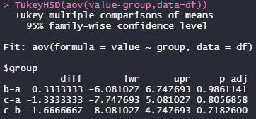

解釈：Pが0.05以下なら平均に差がある

Pairwise t-test

value <- c(5,6,4,6,8,2,3,1,7)
group <- c("a","a","a","b","b","b","c","c","c")
pairwise.t.test(x=value,g=group,data=df, p.adj="bonferroni")
# p.adj = bonferroni, Hochberg, hommel

Pairwise comparisons using t tests with pooled SD
data: value and group

a b
b 1 –
c 1 1

P value adjustment method: bonferroni

解釈：Pが0.05以下なら平均に差がある

３－２－２
３群以上（非正規分布） or（非等分散）Kruskal-Wallis test

value <- c(5,6,4,6,8,2,3,1,7)
group <- c("a","a","a","b","b","b","c","c","c")
df <- tibble(value,group)
kruskal.test(value~group,data=df)

Kruskal-Wallis rank sum test
data: value by group
Kruskal-Wallis chi-squared = 0.69468, df = 2, p-value = 0.7066

解釈：Pが0.05以下なら平均に差がある

Kruskal-Wallis rank sum testの後、どの群に差があったのかを調べる
pairwise Wilcoxon rank-sum tests

value <- c(5,6,4,6,8,2,3,1,7)
group <- c("a","a","a","b","b","b","c","c","c")
pairwise.wilcox.test(x=value,g=group,data=df, p.adj="bonferroni")
# p.adj = bonferroni, Hochberg, hommel

Pairwise comparisons using Wilcoxon rank sum test with continuity correction
data: value and group

a b
b 1 –
c 1 1

P value adjustment method: bonferroni

解釈：Pが0.05以下なら平均に差がある

３－３　正規分布のテスト

３－３－１　サンプル5000件以下　Shapiro-Wilk test

value <- c(5,6,4,6,8,2,3,1,7)
shapiro.test(value)

Shapiro-Wilk normality test
data: value
W = 0.96816, p-value = 0.8785

解釈：p-valueが0.05以上なら正規分布している

３－３－２　その他　Kolmogorov-Smirnov test

value <- c(5,6,4,6,8,2,3,1,7)
ks.test(value,"pnorm",mean = mean(value), sd=sd(value))

One-sample Kolmogorov-Smirnov test
data: value
D = 0.15961, p-value = 0.9759
alternative hypothesis: two-sided

解釈：p-valueが0.05以上なら正規分布している

３－4．等分散のテスト

正規分布が前提条件

３－４－１．F-test　条件：２群＆正規分布

value <- c(5,6,4,6,8,2)
group <- c("a","a","a","b","b","b")
df <- tibble(value,group)
var.test(value~group,data=df)

F test to compare two variances
data: value by group
F = 0.10714, num df = 2, denom df = 2, p-value = 0.1935
alternative hypothesis: true ratio of variances is not equal to 1
95 percent confidence interval:
0.002747253 4.178571429
sample estimates:
ratio of variances
0.1071429

解釈：p-valueが0.05以上なら差がない（等分散）

３－４－２．Bartlett’test　条件：３群以上＆正規分布

value <- c(5,6,4,6,8,2,3,1,7)
group <- c("a","a","a","b","b","b","c","c","c")
df <- tibble(value,group)
bartlett.test(value~group,data=df)

Bartlett test of homogeneity of variances
data: value by group
Bartlett’s K-squared = 1.9207, df = 2, p-value = 0.3828

解釈：p-valueが0.05以上なら差がない（等分散）

４．比率の差の検定

４－１　サンプル５以上・迅速な計算　Pearson’s Chi-squared test

x <- matrix(c(58,99,32,48),nrow=2,ncol=2)
chisq.test(x)

Pearson’s Chi-squared test with Yates’ continuity correction
data: x
X-squared = 0.10054, df = 1, p-value = 0.7512

解釈：p-valueが0.05以下なら差がある

４－２　正確な計算・計算が遅い　Fisher’s Exact Test　

x <- matrix(c(58,99,32,48),nrow=2,ncol=2)
fisher.test(x)

Fisher’s Exact Test for Count Data
data: x
p-value = 0.6728
alternative hypothesis: true odds ratio is not equal to 1
95 percent confidence interval:
0.4886567 1.5906871
sample estimates:
odds ratio
0.8792729

解釈：p-valueが0.05以下なら差がある

４－３　３群以上の比率の比較　

prop.test(c(10,10,10),c(100,200,300))

3-sample test for equality of proportions without
continuity correction

data: c(10, 10, 10) out of c(100, 200, 300)
X-squared = 7.0175, df = 2, p-value = 0.02993
alternative hypothesis: two.sided
sample estimates:
prop 1 　　　prop 2 　　　prop 3
0.10000000 　0.05000000 　0.03333333

解釈：p-valueが0.05以下なら３群の比率は同じではない

なお、同様の結果がカイ二乗検定でも得られる。matrixの作り方が、対象と非対称というように、排他的に作ることに注意。（prop.testでは10/100だが、chisqでは10・90）

chisq.test(matrix(c(10,90,10,190,10,290),nrow=2,ncol=3),correct=T)

Pearson’s Chi-squared test

data: matrix(c(10, 90, 10, 190, 10, 290), nrow = 2, ncol = 3)
X-squared = 7.0175, df = 2, p-value = 0.02993

どの群に差があるか、多群比較をする場合（post hoc test）

pairwise.prop.test(c(10,10,10),c(100,200,300))

Pairwise comparisons using Pairwise comparison of proportions

data: c(10, 10, 10) out of c(100, 200, 300)

　　　1 　　　2
2 　0.328 　　-
3 　0.051 　0.485

P value adjustment method: holm