
第1回:時系列解析の基礎的な関数
第2回:時系列のデータビジュアライゼーション
第3回:時系列の現状分析
第4回:時系列の予想
第5回:予想モデルの評価
使用する言語:R
パッケージ:fpp2(forecast),tidyverse
時系列の予想について
未来の予想をすることが、時系列解析の大きな目的です。未来の予想は、説明変数を用いて目的変数を予想します。一般的な機械学習の方法と異なる点は、説明変数の中に過去の目的変数を入れることができるという点です。
目的変数 = f 1 ( 説明変数1 ) + f 2 ( 説明変数2 ) + …..
未来の予想をする方法は、大きく3つの方法に分けることができます。
1.過去の目的変数のみを説明変数に使う
2.過去の目的変数は使わないで他の変数を説明変数に使う
3.過去の目的変数と、他の変数を説明変数に使う
私は機械学習から学習を始めたのですが、1のような考え方があるのだと目から鱗でした。2は見慣れた方法だと思います。3がわくわくしますね。時系列解析の勉強をすると、多くの方法が1に分類されます。機械学習とは別ルートで発展してきた分野なのでしょう。
1.過去の目的変数のみを説明変数に使う手法
よくわからないけどとりあえず予想したい場合は、ets、arimaあたりを使ったらいいと思います。それも端折りたい場合には、forecast(tsオブジェクト, h = 10)で自動でいいモデルで予想してくれます。
1-1.Regressionを使用した予想
Trendをdecomposeで得て、season(曜日等)をdummy variableとします。それらを説明変数として予測します。
tslm_fit = tslm(tsオブジェクト~trend+season, data=tsオブジェクト)
y~xでregressionの計算式を指定しますが、時系列データが1種のデータだけだとyに相当するものがないので、tsオブジェクト名を入れます。
1-2.Dynamic harmonic regressionを用いた予測
Regressionを実施する際に長い季節期間がある場合には、フーリエ項を季節ダミー変数の変わりに用いると、多くの場合モデルの精度があがります。この手法をharmonic regressionと呼びます。季節ダミー変数を使う代わりに、フーリエ項(cosineとsineの組み合わせ)を使うと、季節ダミー変数の削減ができます。さらに、フーリエ項とARIMAを組み合わせたモデルは、Dynamic harmonic regressionと呼びます。長い季節期間とは、日ごとのデータのように365の期間があったり、週ごとのデータで約52の季節期間の場合などを指します。
dynamic_harmonic_regression = auto.arima(tsオブジェクト, xreg = fourier(tsオブジェクト, K = 2)) # kはフーリエ項の最大数
1-3.Exponential smoothingを使用した予想
指数平滑法は、最も成功した予測法の1つです。指数平滑法による予測は、過去の観測値を加重平均したもので、観測値が古いほど加重は指数関数的に減少していきます。言い換えれば、最近の観測値ほど重みが高くなります。エラー項、トレンド項、sesonal項の組み合わせを指定し、それぞれの項の係数を推測します。
ETS (Error, Trend, Seasonal)
Error: N(None) or A(Additive) or Ad(Additive damped)
Trend: N(None) or A(Additive) or M(multiplicative)
Seasonal: N(None) or A(Additive) or M(multiplicative)
ets_fit = ets(tsオブジェクト)
ETSの組み合わせを指定しない場合には、自動でAICc(corrected Akaike’s Information Criterion)を最小にする最適な項の組み合わせを見つけます。
etsの特別な場合が以下の予測法
- Simple exponential smoothing
ses_fit = ses(tsオブジェクト, h = 10) # forecastを含みます。hは、どれくらい先まで予想するかです。
- Holt’s linear trend method
holt_fit = holt(tsオブジェクト, h = 10) # forecastを含みます。hは、どれくらい先まで予想するかです。
- Holt-Winters’ seasonal method
hw_fit = hw(tsオブジェクト, h = 10) # forecastを含みます。hは、どれくらい先まで予想するかです。
1-4.Seasonal ARIMA models(SARIMA)を使用した予想
ETSモデルとARIMAモデルは、時系列予測に最も広く使われている2つのアプローチです。ARIMA (AutoRegressive Integrated Moving Average)integratedは、差分を元に戻すプロセスを指しています。自行相関項(p)、差分項(d)、移動平均項(q)の組み合わせを指定し、それぞれの項の係数を推測します。
Seasonal ARIMA model:ARIMA( p,d,q ) ( P,D,Q )m
Non – season part ( p,d,q )
p: どれくらいまでの過去データを使うか。p=2なら、時点tの予測をする際に時点t-1と時点t-2のデータを使う。
d: 定常状態に変形する際のパラメータ。時点tと時点t+nの差を計算する際のnの大きさ。通常0か1か2。
q: どれくらいまで、過去の予想と観測値の違い(residual)のデータを使うか。q=2なら、1つ前のresidualと2つ前のresidualを使用する。
Season part( P,D,Q )
P: どれくらいまでの過去データを使うか。p=2なら、時点tの予測をする際に時点t-1と時点t-2のデータを使う。
D: 定常状態に変形する際のパラメータ。時点tと時点t+nの差を計算する際のnの大きさ。通常0か1か2。
Q: どれくらいまで、過去の予想と観測値の違い(residual)のデータを使うか。q=2なら、1つ前のresidualと2つ前のresidualを使用する。
M は、frequencyです。年間の観測回数。
arima_fit = auto.arima(tsオブジェクト)
AICcを小さくする最適な組み合わせを自動で計算してくれます。
arimaの特別な場合が以下の予測法になる。
natural cubic smoothing splines:ARIMA(0,2,2)
natural_cubic_splines = splinef(tsオブジェクト, h = 10) # 予測を含む
1-5.TBATS modelsを使用した予想
フーリエ項とETSおよびBox-Cox変換を組み合わせた方法です。
TBATSモデルとDynamic harmonic regressionとの違いは、harmonic regressionの項が季節パターンを変化させずに周期的に繰り返させるのに対し、TBATSモデルでは季節性が時間とともにゆっくりと変化するようになっている点です。TBATSモデルの欠点は、特に長い時系列の場合、推定に時間がかかることです。
tbats_fit = tbats(tsオブジェクト)
1-6.バギング法による予測
与えられた時系列のデータをSTL分解して、residualsだけをランダムに変化させると、元の時系列によく似た新たな時系列データが手に入ります。Residualsは、もともとランダムですので、新たに得た時系列データも、元の時系列データも本質は同じはずです。このように新たに似た時系列データを作り出し、それを基にモデルを作り、複数の得られた予測を平均化すると、元の時系列を単に直接予測する場合よりも良い予測が得られます。これは、”bootstrap aggregating “の略である “bagging “と呼ばれています。
ETSだけ、バギング用の特別な関数が用意されています。
bagged_ets_fit = baggedETS(tsオブジェクト)
その他の推定方法は、以下の関数で行います。fnに使いたい関数を指定します。以下の場合はauto.arimaです。
bagged_arima_fit = baggedModel(tsオブジェクト, bootstrapped_series = bld.mbb.bootstrap(tsオブジェクト,3),fn=auto.arima)
1-7.STL decompositionを使用した予測
時系列を分解し、季節成分と季節調整成分を別々に予測します。予測の方法には複数手法の中から1つを選ぶ事ができます。
stlf_fit = stlf(tsオブジェクト, method = , h = 10) # forecastを含む
methods には、”ets”, “arima”, “naive”, “rwdrift”のいずれかを指定できます。デフォルトはetsです。
1-8.Neural network autoregressionを用いた予測
Neural networkに過去のデータを入れたモデル。
NNAR( p,P,k ) mで表現されます。
m:frequency。年間の観測回数。
k:ニューロンの数
P:どれくらいまでの過去のfequencyを使うか。M=12、P=2なら、時点tから12時点前と、24時点前のデータを使う。
p:どれくらいまでの過去データを使うか。p=2なら、時点tの予測をする際に時点t-1と時点t-2のデータを使う。
neural_network_fit = nnetar(tsオブジェクト) # xregも指定可
自動で、AICが最小の上記のパラメーターを算出します。
1-9.そのほかの単純な予測方法
単純だけど、意外と精度が高くなるらしいです。ベースのモデルとして、使われます。作ったモデルが、これらより精度がよくないと悲しいです。
- 平均法
将来のすべての値の予測が、過去のデータの平均値。
mean_fit = meanf(tsオブジェクト, h = 10) # forecastを含む
- Naïve method
単純にすべての予測を最後の観測値とします
naive_fit = naive(tsオブジェクト, h = 10) # forecastを含む
- Seasonal naïve method
各予測値は、その年の同じ季節(例:前年の同じ月)に観測された最後の値と同じです。
snaive_fit = snaive(tsオブジェクト, h = 10) # forecastを含む
- Drift method
最初の観測値と最後の観測値の間に線を引き、それを未来に向かって外挿して予測します。
rwf_with_drift = rwf(tsオブジェクト, drift = T, h = 10) # forecastを含む
2.過去の目的変数は使わないで他の変数を説明変数に使う手法
Regression:説明変数は他の変数
tslm_fit = tslm(目的変数~説明変数, data=tsオブジェクト)
将来を予測する場合には、未来の説明変数の値を設定する必要があります。newdataとして、forecastの際に指定します。newdataはdataframeで作らないといけません。
例1:説明変数の平均を使い続ける
new説明変数 <- data.frame(説明変数 = rep(mean(説明変数), 10))
forecast(tslm_fit, newdata=new説明変数)
例2:予測した説明変数の値を使う
new説明変数 <- data.frame(説明変数 = forecast(ets(説明変数), h=10)$mean)
forecast(tslm_fit, newdata=new説明変数)
3.過去の目的変数と、他の変数を説明変数に使う手法
Dynamic regression:説明変数は他の変数 + 目的変数の過去データ
SARIMAのモデルは通常目的変数の過去データのみを使って予測を行いますが、他の説明変数を組み込むこともできます。
まず、説明変数のtsオブジェクトを作る必要があります。
説明変数が1つだけのとき
xreg <- (patient = tsオブジェクト[ ,”説明変数”])
説明変数が2つ以上のとき
xreg <- cbind( x1 = .. , x2 = …)
dynamic_regression_fit = auto.arima(tsオブジェクト[ ,”目的変数”], xreg=xreg)
予想するときは、未来の説明変数の値を設定する必要があります。
newxreg <- (patient = rep(mean(tsオブジェクト[ ,”目的変数”]), 10))
forecast(dynamic_regression_fit, xreg=newxreg)
Dynamic regression:説明変数は他の変数のlag variables+ 目的変数の過去データ
lag variablesは広告などの効果が後になって現れるような現象を考慮に入れたものです。過去の説明変数の数値を使います。基本は上のやり方と同じですが、説明変数のtsオブジェクトを作る際に苦労があります。
例として、7日間のラグ変数、さらに、未来の説明変数を予想したものを使います。
xreg <- cbind(説明変数 = tsオブジェクト[,"説明変数"],
              lag1説明変数 = stats::lag(tsオブジェクト[,"説明変数"],-1),
              lag2説明変数 = stats::lag(tsオブジェクト[,"説明変数"],-2),
              lag3説明変数 = stats::lag(tsオブジェクト[,"説明変数"],-3),
              lag4説明変数 = stats::lag(tsオブジェクト[,"説明変数"],-4),
              lag5説明変数 = stats::lag(tsオブジェクト[,"説明変数"],-5),
              lag6説明変数 = stats::lag(tsオブジェクト[,"説明変数"],-6),
              lag7説明変数 = stats::lag(tsオブジェクト[,"説明変数"],-7))%>%
  head(nrow(tsオブジェクト))

dynamic_regression_fit = auto.arima(tsオブジェクト[,"目的変数"][8:nrow(xreg)],
                                    xreg=xreg[8:nrow(xreg),]) # NAのところを避ける


forecast_xreg <- forecast(tsオブジェクト[,"説明変数"], h = 10)

newxreg <- cbind(説明変数 = forecast_xreg$mean,
                 lag1説明変数 = c(tsオブジェクト[NROW(tsオブジェクト),"説明変数",drop=F],stats::lag(forecast_xreg$mean,-1))[1:10],
                 lag2説明変数 = c(tsオブジェクト[(NROW(tsオブジェクト)-1):NROW(tsオブジェクト),"説明変数"],stats::lag(forecast_xreg$mean,-2))[1:10],
                 lag3説明変数 = c(tsオブジェクト[(NROW(tsオブジェクト)-2):NROW(tsオブジェクト),"説明変数"],stats::lag(forecast_xreg$mean,-3))[1:10],
                 lag4説明変数 = c(tsオブジェクト[(NROW(tsオブジェクト)-3):NROW(tsオブジェクト),"説明変数"],stats::lag(forecast_xreg$mean,-4))[1:10],
                 lag5説明変数 = c(tsオブジェクト[(NROW(tsオブジェクト)-4):NROW(tsオブジェクト),"説明変数"],stats::lag(forecast_xreg$mean,-5))[1:10],
                 lag6説明変数 = c(tsオブジェクト[(NROW(tsオブジェクト)-5):NROW(tsオブジェクト),"説明変数"],stats::lag(forecast_xreg$mean,-6))[1:10],
                 lag7説明変数 = c(tsオブジェクト[(NROW(tsオブジェクト)-6):NROW(tsオブジェクト),"説明変数"],stats::lag(forecast_xreg$mean,-7))[1:10])

forecast(dynamic_regression_fit,h=10,xreg=newxreg)
実際に予測してみる
時系列解析の手法を用いて、コロナ患者の数を予想します。疫学的なモデル(SIRモデル)を用いて予想するのがセオリーなのでしょうが、他分野の技術を使ってみます。
使用データ:厚生労働省オープンデータ(https://www.mhlw.go.jp/stf/covid-19/open-data.html)を改変
まずデータを読み込みます。2020年1月16日(土)~2021年3月22日(月)までのデータを使用します。
library(tidyverse)
library(fpp2)
patient <- read.csv("C:\\Users\\pcr_positive_daily.csv",encoding="UTF-8")
colnames(patient) <- c("date","pcr_positive")
patient_ts <- ts(patient$pcr_positive,start = c(1,7), frequency = 7)
autoplot(patient_ts)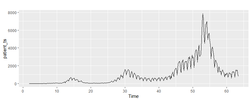
Regression
tslm_trend_season_fit = tslm(patient_ts~trend+season, data=patient_ts)
autoplot(patient_ts)+
  autolayer(tslm_trend_season_fit$fitted.values)+
  autolayer(forecast(tslm_trend_season_fit,h=10),series="Autoregression\nvariables = trend,  season")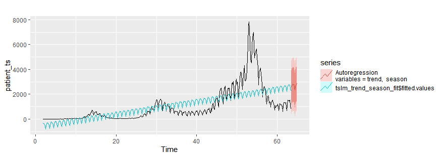
Dynamic harmonic regression
dynamic_harmonic_regression = auto.arima(patient_ts, xreg = fourier(patient_ts, K = 2))
autoplot(patient_ts)+
  autolayer(dynamic_harmonic_regression$fitted)+
  autolayer(forecast(dynamic_harmonic_regression, xreg=fourier(patient_ts, K = 2, h=10)),series="Dynamic harmonic regression")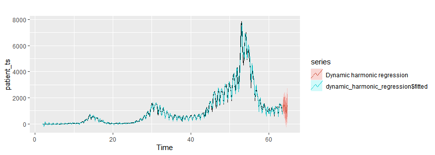
Exponential smoothing
ets_fit = ets(patient_ts)
autoplot(patient_ts)+
  autolayer(ets_fit$fitted)+
  autolayer(forecast(ets_fit,h=10),series="exponential smoothing methods")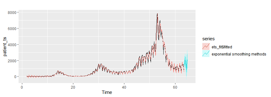
Simple exponential smoothing
ses_fit = ses(patient_ts, h=10)
autoplot(patient_ts)+
  autolayer(ses_fit$fitted)+
  autolayer(ses_fit,series="Simple exponential smoothing")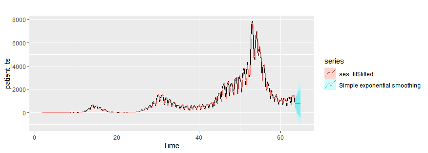
Holt’s linear trend method
holt_fit = holt(patient_ts, h=10)
autoplot(patient_ts)+
  autolayer(holt_fit$fitted)+
  autolayer(holt_fit,series="Holt’s linear trend method")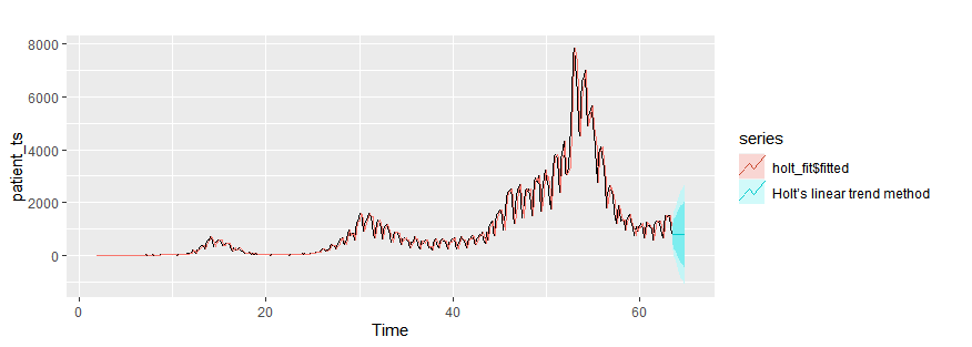
Holt-Winters’ seasonal method
hw_fit = hw(patient_ts, h=10)
autoplot(patient_ts)+
  autolayer(hw_fit$fitted)+
  autolayer(hw_fit,series="Holt-Winters’ method")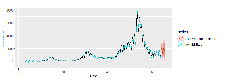
Seasonal ARIMA models
arima_fit = auto.arima(patient_ts)
autoplot(patient_ts)+
  autolayer(arima_fit$fitted)+
  autolayer(forecast(arima_fit,h=10),series="ARIMA")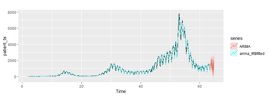
Natural cubic smoothing splines
natural_cubic_splines = splinef(patient_ts, h=10)
autoplot(patient_ts)+
  autolayer(natural_cubic_splines$fitted)+
  autolayer(forecast(natural_cubic_splines,h=10),series="natural_cubic_splines")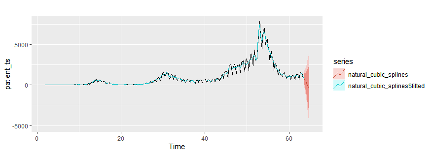
TBATS models
tbats_fit = tbats(patient_ts)
autoplot(patient_ts)+
  autolayer(tbats_fit$fitted.values)+
  autolayer(forecast(tbats_fit,h=10),series="TBATS")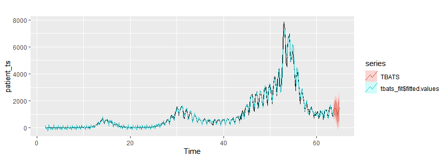
Bagging ETS
bagged_ets_fit = baggedETS(patient_ts)
autoplot(patient_ts)+
  autolayer(bagged_ets_fit$fitted)+
  autolayer(forecast(bagged_ets_fit,h=10),series="Bagged ETS")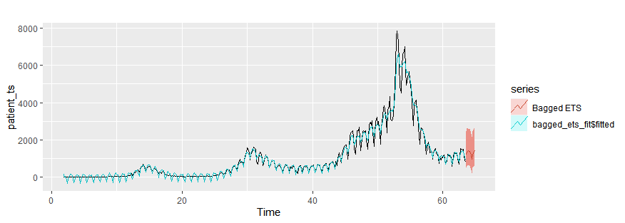
Bagging auto ARIMA
bagged_arima_fit = baggedModel(patient_ts, bootstrapped_series = bld.mbb.bootstrap(patient_ts,3),fn=auto.arima)
autoplot(patient_ts)+
  autolayer(bagged_arima_fit$fitted)+
  autolayer(forecast(bagged_arima_fit,h=10),series="Bagged ARIMA")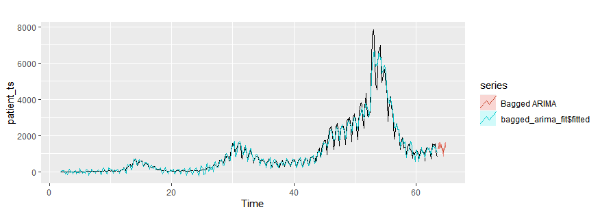
STL decomposition
stlf_fit = stlf(patient_ts, h=10) # method = "ets"
autoplot(patient_ts)+
  autolayer(stlf_fit$fitted)+
  autolayer(stlf_fit,series="Seasonal and Trend decomposition\nusing Loess forecast")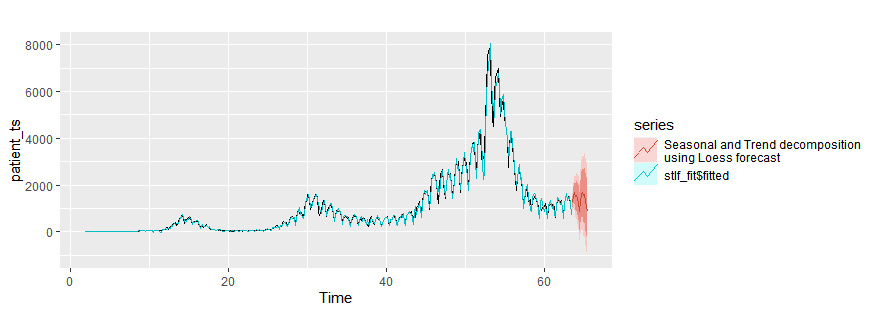
Neural network autoregression
forecastの際にPrediciton Intervalが必要な場合には、PI = Tを入れます。
neural_network_fit = nnetar(patient_ts)
autoplot(patient_ts)+
  autolayer(neural_network_fit$fitted)+
  autolayer(forecast(neural_network_fit,h=10,PI=T),series="Neural Network")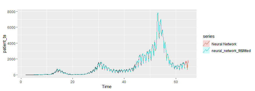
平均法
mean_fit = meanf(patient_ts, h=10)
autoplot(patient_ts)+
  autolayer(mean_fit$fitted)+
  autolayer(mean_fit,series="Average method")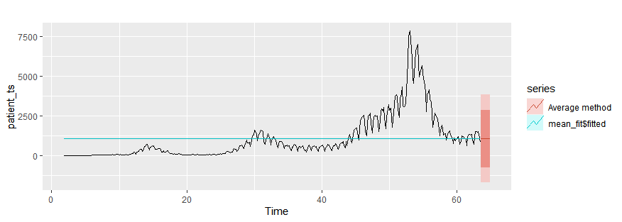
Naïve method
naive_fit = naive(patient_ts, h=10)
autoplot(patient_ts)+
  autolayer(naive_fit$fitted)+
  autolayer(naive_fit,series="Naïve method")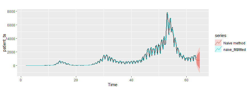
Seasonal naïve method
snaive_fit = snaive(patient_ts, h=10)
autoplot(patient_ts)+
  autolayer(snaive_fit$fitted)+
  autolayer(snaive_fit,series="Seasonal naïve method")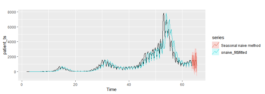
Drift method
rwf_with_drift = rwf(patient_ts, h=10, drift = T)
autoplot(patient_ts)+
  autolayer(rwf_with_drift$fitted)+
  autolayer(rwf_with_drift,series="Drift method")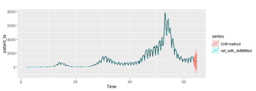
Regression:過去の目的変数は使わないで他の変数を説明変数に使う
例:コロナ死者数を目的変数として、患者数を説明変数とした場合
使用データ:厚生労働省オープンデータ(https://www.mhlw.go.jp/stf/covid-19/open-data.html)を改変
データを読み込みます。2020年2月14日(日)~2021年3月22日(月)までの死者数合計データを使用します。
# コロナ死亡者数合計データを読み込む
death <- read.csv("C:\\Users\\death.csv",encoding="UTF-8")
colnames(death) <-c("date","death")
death$date <- as.Date(death$date, format="%Y/%m/%d")
tsdeath <- ts(death$death,start = c(1,1),frequency = 7)
autoplot(tsdeath)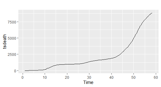
1日の新規死亡者数を計算します
# 1日の新規死亡者数を計算する
diff1 <- diff(tsdeath,d=1)
autoplot(diff1)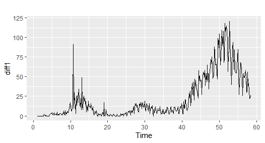
1日後との新規感染者数データとjoinする。
patient <- read.csv("C:\\Users\\pcr_positive_daily.csv",encoding="UTF-8")
colnames(patient) <- c("date","pcr_positive")
patient$date <- as.Date(patient$date, format="%Y/%m/%d")
death_patient <- left_join(death,patient, by = "date")
death_patient$diff <- c(NA,base::diff(death_patient$death,lag = 1))
death_patient_ts <- ts(death_patient,start = c(1,1), frequency = 7)
Regressionをフィットさせる
tslm_fit = tslm(diff~pcr_positive, data=death_patient_ts)forecastで将来を予想する場合には、新規感染者数の予想を与えなければならないです。dataframeで将来の新規感染者数データを作ります。
# 戦略1:過去の平均
newdata1 <- data.frame(pcr_positive = rep(mean(death_patient_ts[,"pcr_positive"]), 10))
autoplot(death_patient_ts[,"diff"])+ autolayer(forecast(tslm_fit,newdata=newdata1),
                                               series = "Regression")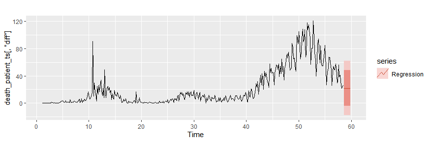
# 戦略2:予測した数値
newdata2 <- data.frame(pcr_positive = forecast(death_patient_ts[,"pcr_positive"],h=10)$mean)
autoplot(death_patient_ts[,"diff"])+ autolayer(forecast(tslm_fit,newdata=newdata2),
                                               series = "Regression")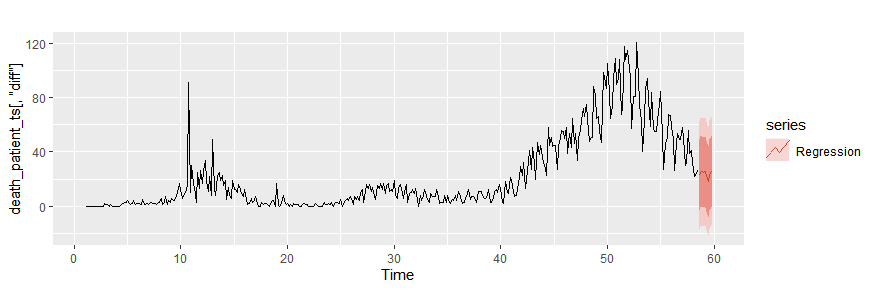
3.過去の目的変数と、他の変数を説明変数に使う手法
Dynamic regression
説明変数のデータ(xreg)をtsオブジェクトで作成する必要があります。
# xregをcbindで作らないといけない。説明変数だけでいい。
xreg <- (patient = death_patient_ts[,"pcr_positive"])

dynamic_regression_fit = auto.arima(death_patient_ts[,"diff"],
                                    xreg=xreg)
# 将来のxregを作成する。過去の平均を使う。
newxreg <- (patient = rep(mean(death_patient_ts[,"pcr_positive"]), 10))
# newxreg <- cbind( x1 = .. , x2 = ...)
autoplot(death_patient_ts[,"diff"])+ autolayer(forecast(dynamic_regression_fit,
                                                        xreg=newxreg),
                                               series = "Dynamic regression")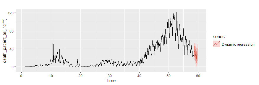
Dynamic regression:説明変数は他の変数のlag variables+ 目的変数の過去データ
# dynamic regression with lag
# lag varibalesを作成
xreg <- cbind(patient = death_patient_ts[,"pcr_positive"],
              lag1patient = stats::lag(death_patient_ts[,"pcr_positive"],-1),
              lag2patient = stats::lag(death_patient_ts[,"pcr_positive"],-2),
              lag3patient = stats::lag(death_patient_ts[,"pcr_positive"],-3),
              lag4patient = stats::lag(death_patient_ts[,"pcr_positive"],-4),
              lag5patient = stats::lag(death_patient_ts[,"pcr_positive"],-5),
              lag6patient = stats::lag(death_patient_ts[,"pcr_positive"],-6),
              lag7patient = stats::lag(death_patient_ts[,"pcr_positive"],-7))%>%
  head(nrow(death_patient_ts))

# モデルをフィットさせる
dynamic_regression_fit = auto.arima(death_patient_ts[,"diff"][8:nrow(xreg)],
                                    xreg=xreg[8:nrow(xreg),]) # NAのところを避ける

# 未来のlag varibalesを作成
forecast_xreg <- forecast(death_patient_ts[,"pcr_positive"], h = 10)

newxreg <- cbind(patient = forecast_xreg$mean,
                 lag1patient = c(death_patient_ts[NROW(death_patient_ts),"pcr_positive",drop=F],stats::lag(forecast_xreg$mean,-1))[1:10],
                 lag2patient = c(death_patient_ts[(NROW(death_patient_ts)-1):NROW(death_patient_ts),"pcr_positive"],stats::lag(forecast_xreg$mean,-2))[1:10],
                 lag3patient = c(death_patient_ts[(NROW(death_patient_ts)-2):NROW(death_patient_ts),"pcr_positive"],stats::lag(forecast_xreg$mean,-3))[1:10],
                 lag4patient = c(death_patient_ts[(NROW(death_patient_ts)-3):NROW(death_patient_ts),"pcr_positive"],stats::lag(forecast_xreg$mean,-4))[1:10],
                 lag5patient = c(death_patient_ts[(NROW(death_patient_ts)-4):NROW(death_patient_ts),"pcr_positive"],stats::lag(forecast_xreg$mean,-5))[1:10],
                 lag6patient = c(death_patient_ts[(NROW(death_patient_ts)-5):NROW(death_patient_ts),"pcr_positive"],stats::lag(forecast_xreg$mean,-6))[1:10],
                 lag7patient = c(death_patient_ts[(NROW(death_patient_ts)-6):NROW(death_patient_ts),"pcr_positive"],stats::lag(forecast_xreg$mean,-7))[1:10])

autoplot(dynamic_regression_fit$x)+
  autolayer(dynamic_regression_fit$fitted)+
  autolayer(forecast(dynamic_regression_fit,h=10,xreg=newxreg))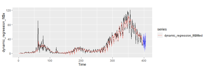
注意事項
Please select a longer horizon when the forecasts are first computed
という表示について。
以下の関数は、関数自体にforecastを含んでいます。特別指定しなければ、h=10です。これらの関数をさらにforecast()で囲み、h = 11以上にすると上のエラーがでます。
meanf()naive()snaive()rwf()stlf()ses()holt()-
hw() splinef()