
前回の続きです。ハンガリーにおけるchikenpox(水疱瘡)のデータを使って、BUTAPESTにおける患者数の3か月分の予想を行っています。前前前回は、AUTOARIMAでMAE36を叩き出しました。前前回は、LightGBMでMAE38でした。今度は、AutoKerasを使って予想したいと思います。前回は、AutokerasでMAE32でした。
今回は
Feature engineering
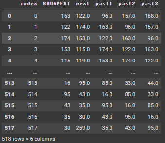
前回と同じですので、省略したいと思います。出来上がりのデータフレームは以下の形です。
TPOT
Scikiet-learnの機械学習ライブラリを使って、遺伝的アルゴリズムにより最適な連鎖処理を見つけることができます。
!pip -q install tpot
from tpot import TPOTRegressor
データをtrain+validation とtestセットに分割します。直近3か月分(13レコード分)を予想したいので、train+validationは最後の13レコードを除いたものにします。また、target variable と explanation variable のデータフレームに分ける必要があります。
X_train_validation = (df4 >> select(~X["next"]))[:-13] # omit target and forecast period
y_train_validation = (df4 >> select(X["next"]))[:-13] # pick up target and omit forecast period
TPOTRegressorオブジェクトを作って、データにフィットさせます。exportで見つけたパイプラインを保存します。
tpot = TPOTRegressor(generations=10,population_size=30, verbosity=2, random_state=42)
tpot.fit(X_train_validation, y_train_validation)
tpot.export("/content/drive/MyDrive/tpot_model.py")
このようなファイルが保存されてます。この1段落目には、データの読み込みをするコードがあります。2段落目にはexported_pipeline = というところに見つけたモデルの情報があります。この1段落目以外の部分をコピペします。
import numpy as np
import pandas as pd
from sklearn.linear_model import ElasticNetCV, RidgeCV
from sklearn.model_selection import train_test_split
from sklearn.neighbors import KNeighborsRegressor
from sklearn.pipeline import make_pipeline, make_union
from sklearn.preprocessing import StandardScaler
from tpot.builtins import StackingEstimator
from tpot.export_utils import set_param_recursive

# NOTE: Make sure that the outcome column is labeled 'target' in the data file
tpot_data = pd.read_csv('PATH/TO/DATA/FILE', sep='COLUMN_SEPARATOR', dtype=np.float64)
features = tpot_data.drop('target', axis=1)
training_features, testing_features, training_target, testing_target = \
            train_test_split(features, tpot_data['target'], random_state=42)

# Average CV score on the training set was: -2687.9116082907785
exported_pipeline = make_pipeline(
    StackingEstimator(estimator=RidgeCV()),
    StandardScaler(),
    StackingEstimator(estimator=KNeighborsRegressor(n_neighbors=30, p=1, weights="uniform")),
    ElasticNetCV(l1_ratio=0.15000000000000002, tol=0.001)
)
# Fix random state for all the steps in exported pipeline
set_param_recursive(exported_pipeline.steps, 'random_state', 42)

exported_pipeline.fit(training_features, training_target)
results = exported_pipeline.predict(testing_features)
時系列データなので、1未来づつ予測します。現在までのレコードで、再学習させます。importの部分は、上のファイルからのコピーです。sklearnからモデルを読み込んでいます。
import numpy as np
import pandas as pd
from sklearn.linear_model import ElasticNetCV, RidgeCV
from sklearn.model_selection import train_test_split
from sklearn.neighbors import KNeighborsRegressor
from sklearn.pipeline import make_pipeline, make_union
from sklearn.preprocessing import StandardScaler
from tpot.builtins import StackingEstimator
from tpot.export_utils import set_param_recursive
# Average CV score on the training set was: -2687.9116082907785
exported_pipeline = make_pipeline(
StackingEstimator(estimator=RidgeCV()),
StandardScaler(),
StackingEstimator(estimator=KNeighborsRegressor(n_neighbors=30, p=1, weights="uniform")),
ElasticNetCV(l1_ratio=0.15000000000000002, tol=0.001)
)
# Fix random state for all the steps in exported pipeline
set_param_recursive(exported_pipeline.steps, 'random_state', 42)
result_tpot = pd.DataFrame(0,
index=np.arange(13),
columns=["pred", "true_diff"])
last30 = len(df4)-13
last = len(df4)
for i in range(last30,last):
X_train = (df4 >> select(~X["next"])).iloc[0:i]
y_train = (df4 >> select(X["next"])).iloc[0:i]
X_test = (df4 >> select(~X["next"])).iloc[i:i+1]
y_test = (df4 >> select(X["next"])).iloc[i:i+1]
exported_pipeline.fit(X_train, y_train)
pred = exported_pipeline.predict(X_test)
result_tpot.iloc[i-(last30),0] = float(pred)
result_tpot.iloc[i-(last30),1] = y_test.values[0,0]
result_tpot["mae"] = abs(result_tpot["true_diff"]-result_tpot["pred"])
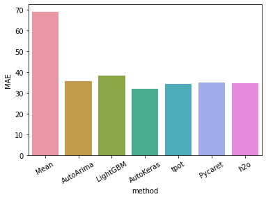
result_tpot["mae"].mean()34.10
AutoMLの結果を比較した表です。Autokerasには負けています。
つぎはpycaretを使って予想をします。